Working with Superphot+

Superphot+ was designed to rapidly fit photometric SN-like light curves to an empirical model for subsequent classification or analysis. This tutorial briefly covers how to import light curves directly from ALeRCE or ANTARES, apply pre-processing for improved quality, and run various sampling methods to fit the light curves.

Light curve import

There are a suite of helper functions in src/data_generation to import photometric light curves from the ALeRCE or ANTARES servers. We will do both here to compare:

[1]:

from dustmaps.config import config

config["data_dir"] = "."  # ensure dustmaps path is correct

# from superphot_plus.file_utils import read_single_lightcurve, save_single_lightcurve
import os
from superphot_plus.constants import *  # all hyperparameters/priors for fitting
from superphot_plus.file_paths import *  # all default file paths, change accordingly
from superphot_plus.utils import *  # all utility functions
from superphot_plus.import_utils import *
from superphot_plus.data_generation.alerce import *
from superphot_plus.data_generation.antares import *

[2]:

test_sn = "ZTF22abvdwik"  # can change to any ZTF supernova

For this tutorial, we will save everything in ../examples/outputs/

[3]:

OUTPUT_DIR = "../examples/outputs/"
os.makedirs(OUTPUT_DIR, exist_ok=True)
generate_single_flux_file(test_sn, OUTPUT_DIR)

../examples/outputs/ZTF22abvdwik.csv

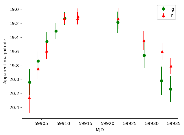
Great! Now let’s extract and plot the lightcurve:

[4]:

import pandas as pd

lc_fn = os.path.join(OUTPUT_DIR, test_sn + ".csv")
df = pd.read_csv(lc_fn)
df

[4]:

	tid	mjd	candid	fid	pid	diffmaglim	isdiffpos	nid	distnr	magpsf	...	magapbig	sigmagapbig	has_stamp	corrected	dubious	step_id_corr	parent_candid	drb	rfid
0	ztf	59902.203692	2148203692115015011	2	2148203692115	20.372300	1	2148	2.014740	20.264100	...	20.1133	0.3801	False	False	False	1.1.6	2.148280e+18	NaN	NaN
1	ztf	59902.280069	2148280062115015013	1	2148280062115	20.216372	1	2148	1.879129	20.042442	...	19.6675	0.2136	True	False	False	1.1.6	NaN	0.995911	650120121.0
2	ztf	59904.178796	2150178792115015047	1	2150178792115	20.618118	1	2150	1.854762	19.739748	...	19.4887	0.1743	True	False	False	1.1.6	NaN	0.999254	650120121.0
3	ztf	59904.196331	2150196332115015044	2	2150196332115	20.588760	1	2150	1.647079	19.854446	...	19.6504	0.2347	True	False	False	1.1.6	NaN	0.998228	650120221.0
4	ztf	59906.152778	2152152772115015009	2	2152152772115	20.328976	1	2152	1.637041	19.599812	...	19.3334	0.1956	True	False	False	1.1.6	NaN	0.999996	650120221.0
5	ztf	59906.199965	2152199962115015019	1	2152199962115	20.751240	1	2152	1.570132	19.463880	...	19.3485	0.1484	True	False	False	1.1.6	NaN	0.999997	650120121.0
6	ztf	59908.238495	2154238492115015017	1	2154238492115	20.428700	1	2154	1.807830	19.313800	...	19.0642	0.1211	False	False	False	1.1.6	2.156177e+18	NaN	NaN
7	ztf	59910.177002	2156177002115015009	2	2156177002115	20.472574	1	2156	1.796709	19.132210	...	19.1670	0.1611	True	False	False	1.1.6	NaN	1.000000	650120221.0
8	ztf	59910.214583	2156214582115015024	1	2156214582115	20.686329	1	2156	1.647136	19.132908	...	18.9604	0.1033	True	False	False	1.1.6	NaN	0.999981	650120121.0
9	ztf	59913.170127	2159170122115015010	2	2159170122115	20.332615	1	2159	1.785321	19.133406	...	19.1690	0.1795	True	False	False	1.1.6	NaN	0.999999	650120221.0
10	ztf	59913.254780	2159254782115015034	2	2159254782115	19.955643	1	2159	1.764815	19.107706	...	18.9649	0.1573	True	False	False	1.1.6	NaN	0.999902	650120221.0
11	ztf	59922.238981	2168238982115015011	1	2168238982115	19.536272	1	2168	1.421017	19.188840	...	18.9854	0.2972	True	False	False	1.1.6	NaN	0.999997	650120121.0
12	ztf	59922.287234	2168287232115015003	2	2168287232115	19.750925	1	2168	1.753629	19.138376	...	19.6920	0.5139	True	False	False	1.1.6	NaN	0.999854	650120221.0
13	ztf	59928.176273	2174176272115015007	2	2174176272115	19.710600	1	2174	1.881800	19.449000	...	18.8682	0.2355	False	False	False	1.1.6	2.174200e+18	NaN	NaN
14	ztf	59928.200428	2174200422115015022	1	2174200422115	20.235287	1	2174	1.974202	19.658592	...	19.2327	0.1603	True	False	False	1.1.6	NaN	0.999430	650120121.0
15	ztf	59932.129618	2178129612115015021	1	2178129612115	20.774820	1	2178	1.599294	20.023670	...	19.8127	0.2198	True	False	False	1.1.6	NaN	0.994586	650120121.0
16	ztf	59932.234479	2178234472115015024	2	2178234472115	20.213923	1	2178	2.010675	19.605530	...	19.4689	0.2228	True	False	False	1.1.6	NaN	0.999785	650120221.0
17	ztf	59934.199630	2180199622115015025	1	2180199622115	20.326313	1	2180	1.784319	20.142624	...	20.4894	0.6155	True	False	False	1.1.6	NaN	0.996885	650120121.0
18	ztf	59934.239526	2180239522115015004	2	2180239522115	20.490465	1	2180	1.810079	19.811592	...	19.8279	0.2983	True	False	False	1.1.6	NaN	0.999997	650120221.0

19 rows × 27 columns

[5]:

import matplotlib.pyplot as plt

m = df["magpsf"]  # magnitudes
merr = df["sigmapsf"]  # mag errs
t = df["mjd"]  # times
b = df["fid"] - 1  # alter so 0=g, 1=r

plt.errorbar(t[b == 0], m[b == 0], yerr=merr[b == 0], fmt="o", c="g", label="g")
plt.errorbar(t[b == 1], m[b == 1], yerr=merr[b == 1], fmt="^", c="r", label="r")

plt.legend()
plt.xlabel("MJD")
plt.ylabel("Apparent magnitude")
plt.gca().invert_yaxis()

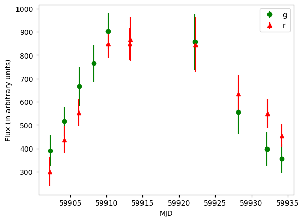
Because our fitting procedure assumes flux units instead of magnitude, we convert using an average zeropoint of 26.3. We also rule out any NaN values, sort the lightcurve, clip bogus LC tails, and apply extinction:

[6]:

t, f, ferr, b, ra, dec = import_lc(lc_fn)

plt.close()
plt.errorbar(t[b == "g"], f[b == "g"], yerr=ferr[b == "g"], fmt="o", c="g", label="g")
plt.errorbar(t[b == "r"], f[b == "r"], yerr=ferr[b == "r"], fmt="^", c="r", label="r")

plt.legend()
plt.xlabel("MJD")
plt.ylabel("Flux (in arbitrary units)")

[6]:

Text(0, 0.5, 'Flux (in arbitrary units)')

We will then save these pre-processed lightcurves as a separate file to be input into the fitting scripts:

[7]:

from superphot_plus.lightcurve import Lightcurve

lc = Lightcurve(
    times=t,
    fluxes=f,
    flux_errors=ferr,
    bands=b,
    name=test_sn,
)
lc.save_to_file(
    os.path.join(OUTPUT_DIR, test_sn+".npz"),
    overwrite=True,
)

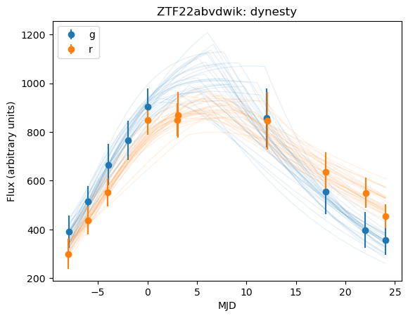
Fitting Light Curves

There are a few sampling techniques implemented for rapid fitting of light curves: * Nested sampling (dynesty) constrains the posterior space with nested ellipsoids of increasing density. * Advanced HMC with the NUTS sampler (using numpyro) uses Hamiltonian Monte Carlo sampling but without U-turns to increase sampling efficiency. * Stochastic variational inference (SVI; also using numpyro) approximates the marginal distributions for each fit as Gaussians, which sacrifices precision for much faster runtime. Recommended for realtime applications.

Let’s use each to fit our test light curve:

[8]:

from superphot_plus.lightcurve import Lightcurve
from superphot_plus.samplers.dynesty_sampler import DynestySampler
from superphot_plus.samplers.numpyro_sampler import NumpyroSampler
from superphot_plus.surveys.surveys import Survey

fn_to_fit = os.path.join(OUTPUT_DIR, test_sn + ".npz")
lightcurve = Lightcurve.from_file(fn_to_fit)
priors = Survey.ZTF().priors

[9]:

%%time

sampler = DynestySampler()
posteriors = sampler.run_single_curve(lightcurve, priors=priors, rstate=np.random.default_rng(9876))
posteriors.save_to_file(OUTPUT_DIR)
print("Nested sampling")

Nested sampling
CPU times: user 1.74 s, sys: 23.2 ms, total: 1.76 s
Wall time: 1.76 s

[10]:

%%time

sampler = NumpyroSampler()
posteriors = sampler.run_single_curve(lightcurve, priors=priors, rng_seed=1, sampler="NUTS")
posteriors.save_to_file(OUTPUT_DIR)
print("NUTS")

Running numpyro with seed=1

sample: 100%|██████████| 1300/1300 [00:03<00:00, 344.09it/s, 31 steps of size 1.81e-01. acc. prob=0.90]

NUTS
CPU times: user 6.16 s, sys: 204 ms, total: 6.36 s
Wall time: 6.3 s

[11]:

%%time

sampler = NumpyroSampler()
posteriors = sampler.run_single_curve(lightcurve, priors=priors, rng_seed=1, sampler="svi")
posteriors.save_to_file(OUTPUT_DIR)
print("SVI")

Running numpyro with seed=1
0
SVI
CPU times: user 3.42 s, sys: 114 ms, total: 3.54 s
Wall time: 3.47 s

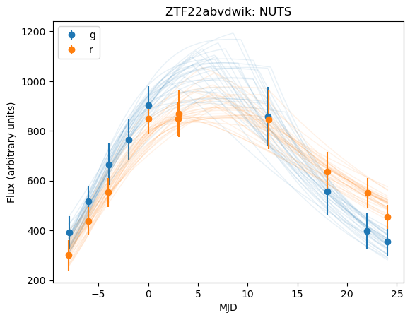
Now, let’s plot each fit to compare results!

[12]:

from superphot_plus.plotting.lightcurves import plot_lc_fit
from IPython import display
from superphot_plus.surveys.surveys import Survey

priors = Survey.ZTF().priors
for method in ["dynesty", "NUTS", "svi"]:
    plot_lc_fit(test_sn, priors.reference_band, priors.ordered_bands, OUTPUT_DIR, OUTPUT_DIR, OUTPUT_DIR, sampling_method=method, file_type="png")

display.Image(os.path.join(OUTPUT_DIR, test_sn + "_dynesty.png"))

[12]:

[13]:

display.Image(os.path.join(OUTPUT_DIR, test_sn + "_NUTS.png"))

[13]:

[14]:

display.Image(os.path.join(OUTPUT_DIR, test_sn + "_svi.png"))

[14]:

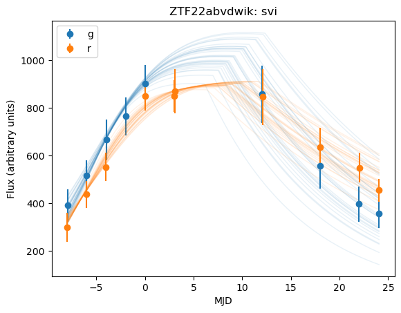
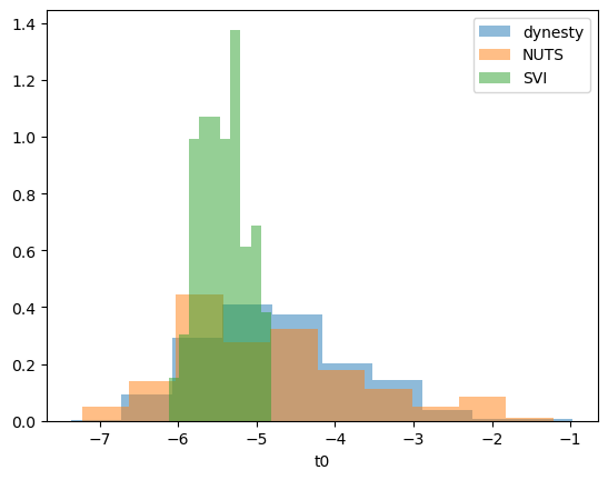
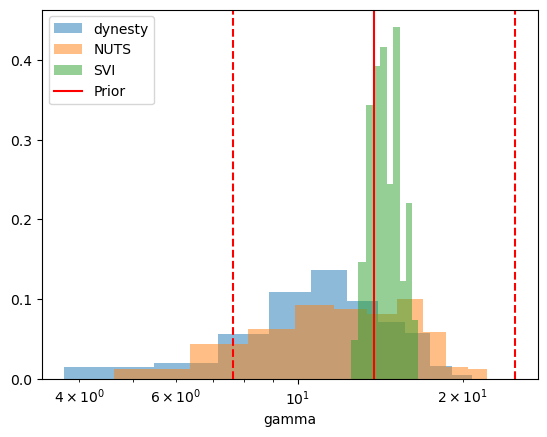
It looks like there is a tradeoff between fit time and fit quality, though there may be an issues with priors. Plotting the distribution for our differing parameters (\(t0\) and \(\gamma\)), we get:

[15]:

params_dynesty = np.load(os.path.join(OUTPUT_DIR, test_sn + "_eqwt_dynesty.npz"))["arr_0"]
# print(params_dynesty[:,-1])
print(params_dynesty[0])
params_NUTS = np.load(os.path.join(OUTPUT_DIR, test_sn + "_eqwt_NUTS.npz"))["arr_0"]
params_svi = np.load(os.path.join(OUTPUT_DIR, test_sn + "_eqwt_svi.npz"))["arr_0"]

t0_idx = 3
gamma_idx = 2

plt.hist(params_dynesty[:, t0_idx], alpha=0.5, label="dynesty", density=True)
plt.hist(params_NUTS[:, t0_idx], alpha=0.5, label="NUTS", density=True)
plt.hist(params_svi[:, t0_idx], alpha=0.5, label="SVI", density=True)
plt.xlabel("t0")
plt.legend()
plt.show()

[ 9.84992253e+02  5.45516161e-03  1.44425585e+01 -6.13319471e+00
  3.56714481e+00  2.92584573e+01  2.23144554e-02  1.03953701e+00
  1.04165270e+00  1.01942523e+00  1.00005030e+00  9.57442160e-01
  5.83623109e-01  8.32112172e-01 -5.45602401e+00]

[16]:

from superphot_plus.surveys.surveys import Survey

ztf_priors = Survey.ZTF().priors
r_priors = ztf_priors.bands["r"]
PRIOR_GAMMA = r_priors.gamma

plt.hist(params_dynesty[:, gamma_idx], alpha=0.5, label="dynesty", density=True)
plt.hist(params_NUTS[:, gamma_idx], alpha=0.5, label="NUTS", density=True)
plt.hist(params_svi[:, gamma_idx], alpha=0.5, label="SVI", density=True)
plt.axvline(10**PRIOR_GAMMA.mean, c="r", label="Prior")
plt.axvline(10 ** (PRIOR_GAMMA.mean + PRIOR_GAMMA.std), c="r", linestyle="dashed")
plt.axvline(10 ** (PRIOR_GAMMA.mean - PRIOR_GAMMA.std), c="r", linestyle="dashed")
plt.xlabel("gamma")
plt.legend()
plt.xscale("log")
plt.show()

Classification

Superphot+ uses the resulting fit parameters as input features for a multi-layer perceptron (MLP) classifier. We can call the classification functions to return probabilities of the object being each of 5 major supernova types:

[17]:

from superphot_plus.utils import adjust_log_dists
from superphot_plus.model.classifier import SuperphotClassifier
from superphot_plus.file_utils import get_posterior_samples
from superphot_plus.file_paths import TRAINED_MODEL_FN, TRAINED_CONFIG_FN

model = SuperphotClassifier.load(TRAINED_MODEL_FN, TRAINED_CONFIG_FN)[0]
lc_probs = model.classify_single_light_curve(test_sn, OUTPUT_DIR, sampler="dynesty")[0]
print(lc_probs)

# Alternatively, classify from posterior samples directly
fit_params = get_posterior_samples(test_sn, OUTPUT_DIR, "dynesty")
# print(params_dynesty[0])
adj_params = adjust_log_dists(fit_params)
lc_probs2 = model.classify_from_fit_params(adj_params)
print(np.subtract(lc_probs, np.mean(lc_probs2, axis=0)))

0.040422052
[ 0.         -0.11821468 -0.36856654 -0.3074244  -0.00368445]

Improvements that need to be made:

Exploration why variation between dynesty + numpyro fits
Quantifying minimum number of iters for SVI or warmup samples for NUTS for asymptotic fitting behavior
Modularizing numpyro script, removal of magic numbers
Refining plotting file, maybe splitting into separate folder

[ ]: